Distribution of Random Vector Length

Distribution of Random Vector Length

In a bout of boredom, I took upon a small R project, as one does. In this project, the main goal was to determine the distribution of a Pythagorean expression, that is Sqrt(A^2 + B^2) where A and B are standard normals.

Some practical application exists for this I'm sure, but at least geometrically it corresponds to the length of a random vector in an AB space.

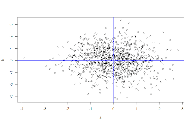
Here is those values, n=1000

n=10000

Without actually doing the transformations by hand, it isn't hard with some background knowledge to see a standard normal squared is a chi-square, the sum of chi-squares is a gamma, and the square root of a gamma is a particular gamma.
A helpful R package lets me sample for gamma parameters and see how close my sampled graphs match.
A smoothed density of sampled distribution over a gamma with the sampled parameters show how close a gamma can fit with our sampled data. n=10000 and 1000 respectively

Shouldn't be a surprise that a gamma is the result, as length is strictly greater than or equal to zero, so a practical application may be how far someone can throw a paper airplane. The actual location can be the distance with a polar uniform distribution, and violà

follow me on twitter @kevgk2 for more blog updates!

Some helpful R code below
 #generate random standard normal values
a<-rnorm(1000,0,1)
b<-rnorm(1000,0,1)

#put into data frame
df<-data.frame(a,b)
View(df)

#do the data transformations, appending data frame
df<-transform(df, sqa = a^2)
df<-transform(df, sqb = b^2)
df<-transform(df, sum = sqa + sqb)
df<-transform(df, sqrsum = sqrt(sum))

#quick summary
summary(df$sqrsum)
   Min. 1st Qu.  Median    Mean 3rd Qu.    Max.
0.05633 0.73086 1.16818 1.23662 1.62847 3.92648

#plot values
plot(a,b)

#add horizontal/vertical lines with specific color
abline(h=mean(df$b), col="blue")
abline(v=mean(df$a), col="blue")

#plot the smoothed histogram of our data
plot(density(df$sqrsum))

#use MASS library for fitdistr command to esitmate gamma paramters
#alternatively use MASS::fitdistr(
library(MASS)
fitdistr(df$sqrsum,'gamma')
     shape       rate 
  3.1351734   2.5352743
 (0.1334236) (0.1170093)

#plot density curve with specific y range so the next curve is within the window
plot(density(df$sqrsum), ylim=c(0,0.7), col = "blue")

#draw the gamma density on our plot copying the parameters above
curve(dgamma(x,shape=3.1351734,rate=2.5352743), from=0,to=5, add = TRUE, col = "red")

#repeat for a larger sample size
c<-rnorm(10000,0,1)
d<-rnorm(10000,0,1)
df2<-data.frame(c,d)
df2<-transform(df2,sqc = c^2)
df2<-transform(df2,sqd = d^2)
df2<-transform(df2,sum=sqc+sqd)
df2<-transform(df2,sqrsum=sqrt(sum))
summary(df2$sqrsum)
   Min. 1st Qu.  Median    Mean 3rd Qu.    Max.
0.02213 0.76682 1.18653 1.26296 1.66958 4.61189
plot(c,d)
abline(h=mean(df2$d),col="blue")
abline(v=mean(df2$c),col="blue")
plot(density(df$sqrsum))
plot(density(df2$sqrsum))
fitdistr(df2$sqrsum,'gamma')
     shape         rate 
  3.18359896   2.52073194
 (0.04287363) (0.03676913)
plot(density(df2$sqrsum), ylim=c(0,0.7),col="blue")
curve(dgamma(x,shape=3.18359896,rate=2.52073194),from=0,to=5,add=TRUE,col="red")